Exploring the Cosmological Redshift from Inhomogeneous Expansion: A Review of the Void–Wall Backreaction Model and New Predictions
Abstract
The Hubble tension—a ~9% discrepancy between the locally measured Hubble constant (H0 ≈ 73 km/s/Mpc from supernovae) and the value inferred from the cosmic microwave background (H0 ≈ 67.4 km/s/Mpc)—remains one of the most pressing problems in modern cosmology. We investigate whether cosmological backreaction, the effect of averaging the Einstein equations over an inhomogeneous universe, can partially account for this discrepancy. Using the Buchert scalar averaging framework and a two-scale void–wall model, we find a local Hubble enhancement of ~2–5%, closing ~25–55% of the tension. In the observationally viable regime with shear corrections, the model provides a ~1–2% correction to the standard ΛCDM prediction. We identify three potentially novel predictions: a directional H0 anisotropy correlated with the tidal field, a redshift drift signature testable with next-generation telescopes, and a structure-enhanced Λ framework distinct from the Wiltshire timescape.
The Hubble Tension
The Hubble constant H0 quantifies the present-day expansion rate of the universe. Two independent methods of measuring it yield discrepant values. The Planck satellite, fitting a homogeneous model to the cosmic microwave background (CMB) radiation from when the universe was ~380,000 years old, gives H0 = 67.4 ± 0.5 km/s/Mpc. Meanwhile, the local distance ladder (SH0ES), using Type Ia supernovae calibrated by Cepheid variable stars within ~300 Mpc, gives H0 = 73.0 ± 1.0 km/s/Mpc.
The discrepancy exceeds 5σ and persists across multiple independent local methods. No consensus resolution exists within the standard ΛCDM cosmological model, which assumes a perfectly homogeneous background geometry.
Inhomogeneous Expansion
The real universe is not homogeneous. Cosmic structure—voids, filaments, walls, and clusters—produces spatial variations in the local expansion rate. Voids expand faster than average; overdense regions expand more slowly or collapse. The standard ΛCDM model ignores this variance in expansion rates by assuming that the average of Einstein’s equations in the inhomogeneous universe equals the Einstein equations evaluated at the average density.
This assumption is not generally valid in general relativity because the Einstein equations are nonlinear: the average of a nonlinear function is not the function of the average. The corrections arising from this nonlinearity are called cosmological backreaction. The question is whether these corrections are large enough to measurably affect H0.
The Buchert Framework
Thomas Buchert (2000) showed that spatially averaging the Einstein equations over a finite domain produces effective Friedmann-like equations with extra source terms absent in the homogeneous case. The key result is the averaged Hamiltonian constraint:
3HD2 = 8πG⟨ρ⟩D − ½⟨R⟩D − ½QD + Λ
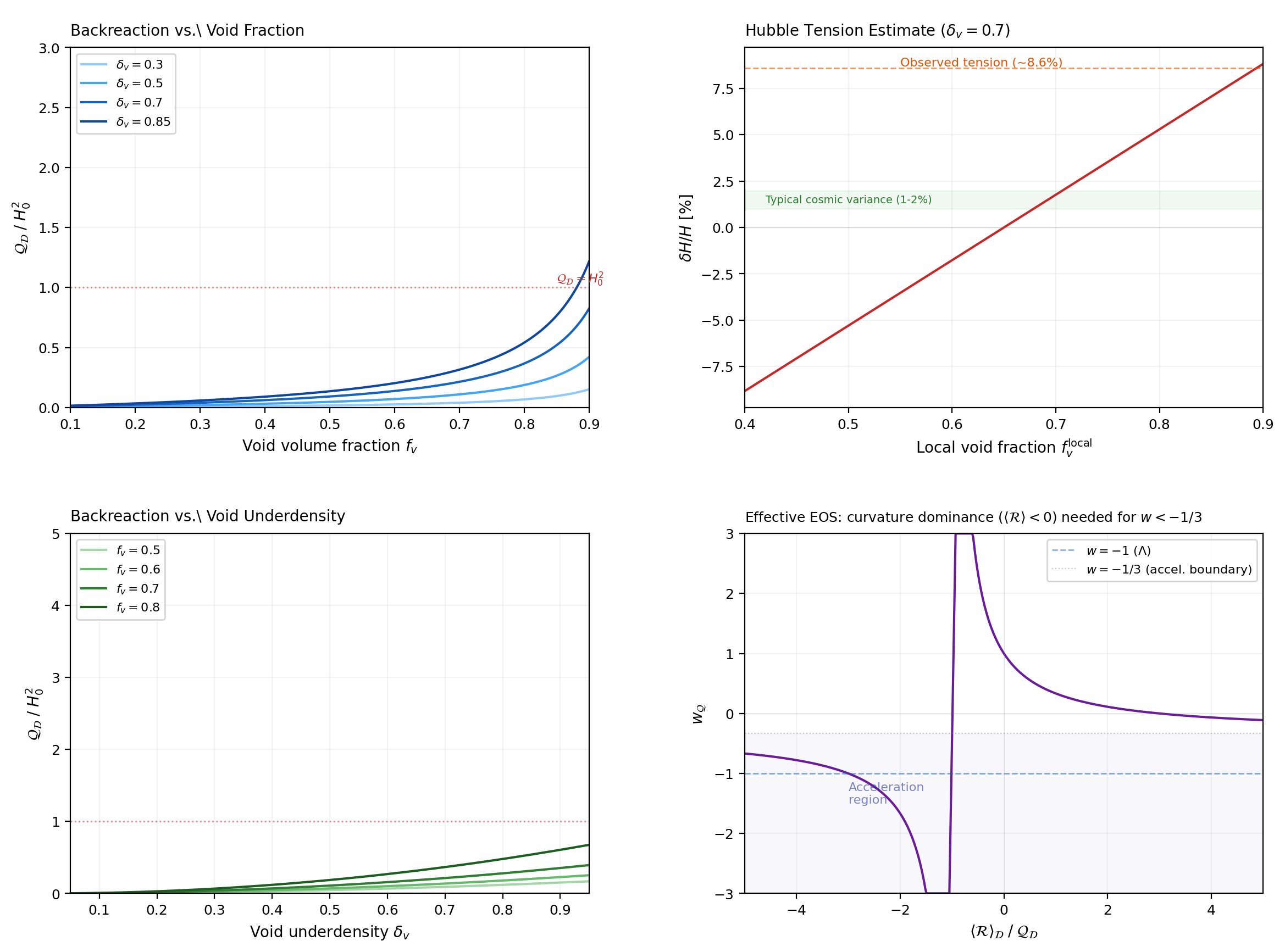
Compared to the standard Friedmann equation, two new terms appear. The kinematical backreaction QD measures the variance in expansion rates across the domain, corrected for shear:
QD = ⅔(Var(θ)) − 2⟨σ2⟩D
And the averaged spatial curvature ⟨R⟩D captures the curvature generated by density contrasts. A critical subtlety: positive QD (from expansion variance) actually reduces the Hubble rate, while negative averaged curvature (from void-dominated geometry) increases it. Curvature is the dynamical lever, not QD directly.
The Two-Scale Void–Wall Model
We partition the universe into two types of regions: voids (underdense, expanding faster) and walls (overdense, expanding slower). Each region evolves according to its own Friedmann equation with its own scale factor and Hubble rate. The domain-averaged Hubble rate is:
HD = fv Hv + fw Hw
where fv and fw are the void and wall volume fractions. The backreaction simplifies to:
QD = 6 fv fw (Hv − Hw)2 ≥ 0
A clean result: the backreaction is proportional to the squared difference in expansion rates between voids and walls, weighted by their volume fractions.
Numerical Results
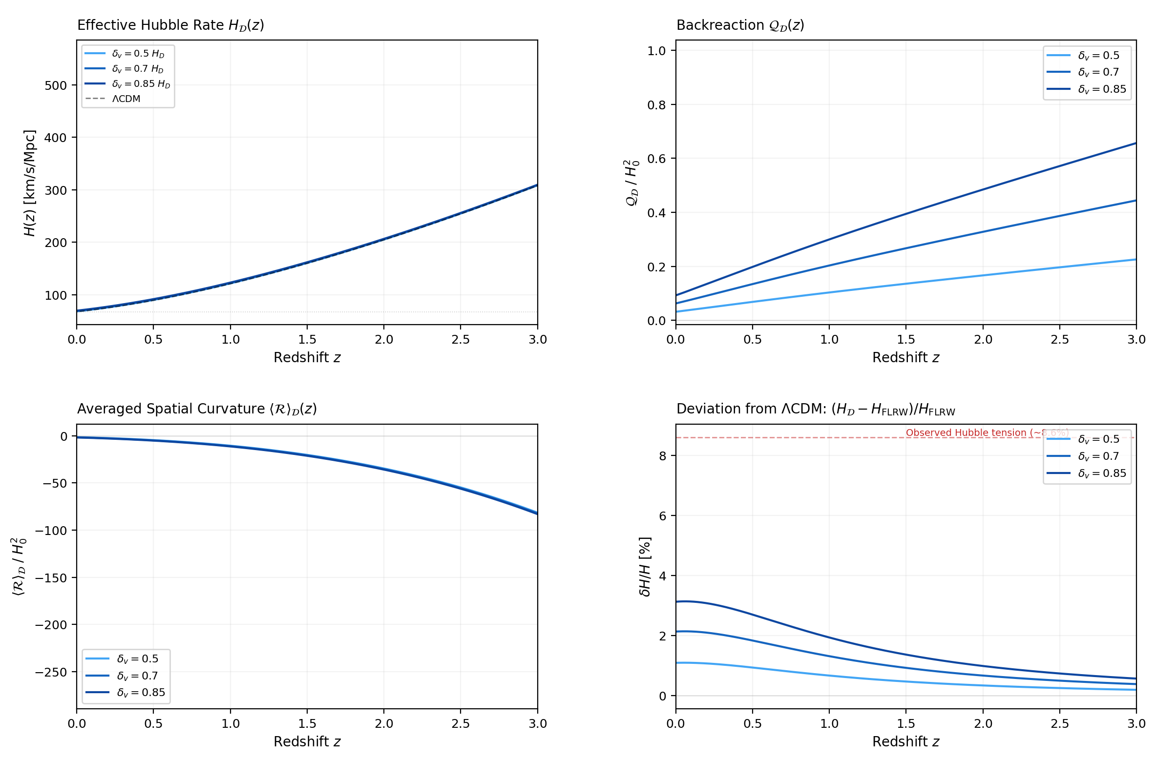
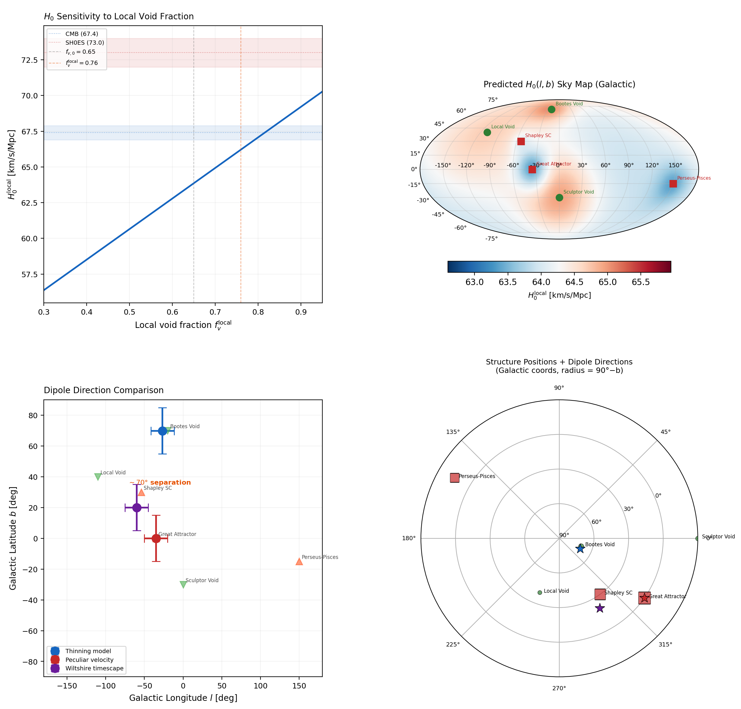
We numerically integrate separate Friedmann equations for void and wall regions from redshift z = 100 to z = 0. Each region has its own density, scale factor, and curvature, evolving self-consistently. The “local” Hubble rate uses an enhanced void fraction (fvlocal = 0.76) to model our position in a region with above-average void content.
| δv tgt | δv act | HD | Hlocal | δHlocal | QD/H02 | ⟨R⟩/H02 |
|---|---|---|---|---|---|---|
| -0.50 | -0.241 | 68.1 | 69.0 | 2.3% | 0.032 | −1.44 |
| -0.70 | -0.313 | 68.8 | 69.8 | 3.6% | 0.063 | −1.62 |
| -0.85 | -0.360 | 69.5 | 70.5 | 4.6% | 0.093 | −1.79 |
All H values in km/s/Mpc. Parameters: fv,0 = 0.65, Ωm = 0.315, H0CMB = 67.4 km/s/Mpc.
Key findings: The backreaction magnitude is QD/H02 ≈ 0.03–0.09, orders of magnitude above perturbative estimates (~10−5) but below the O(1) regime. Curvature dominates: |⟨R⟩|/H02 ≈ 1.4–1.8, far exceeding QD. The local Hubble enhancement δH ≈ 2–5% closes ~25–55% of the Hubble tension.
Observational Comparison
The model must be consistent with existing cosmological data. We compare against three constraints:
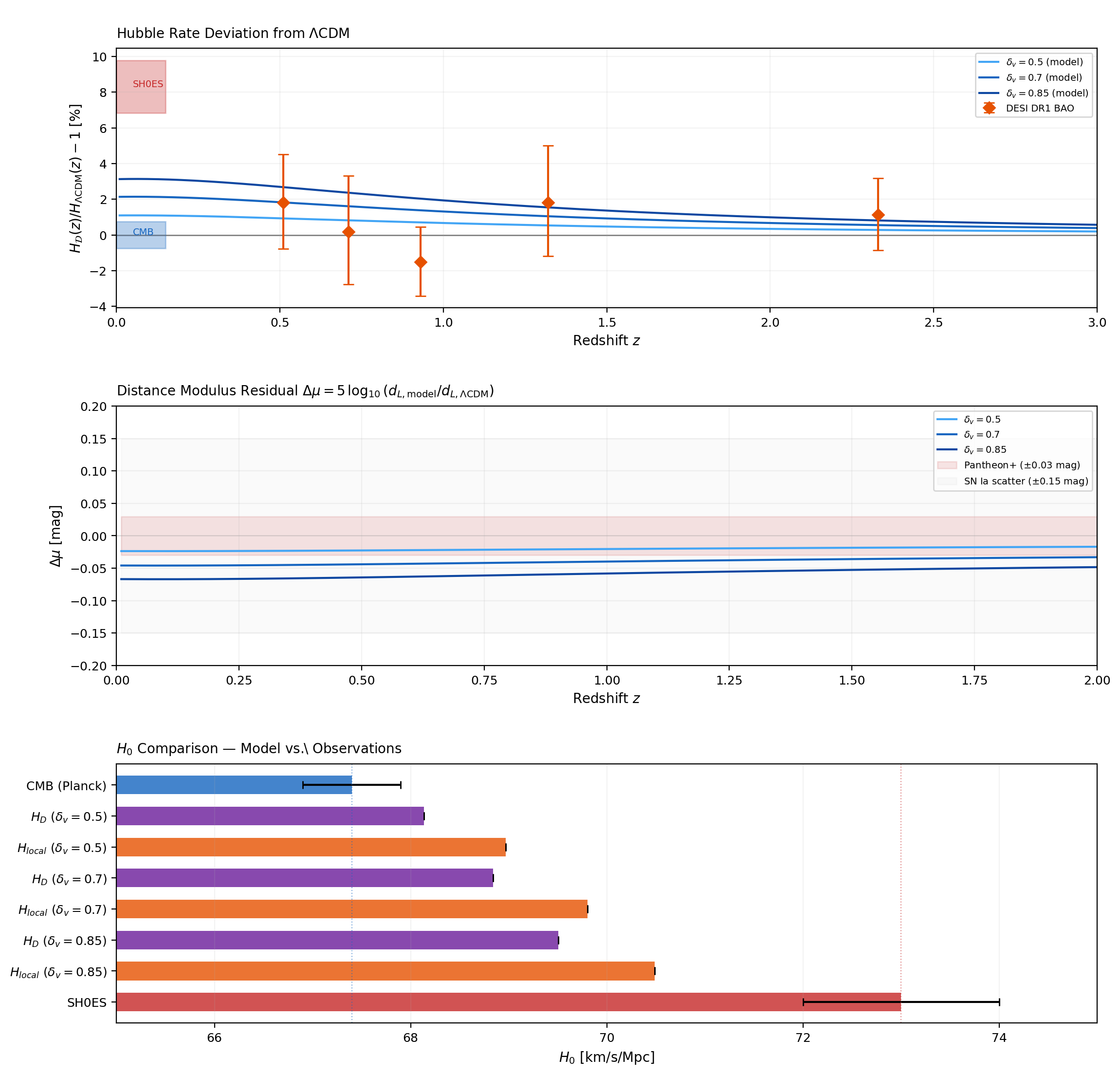
Pantheon+ supernovae: The distance modulus residual Δμ quantifies how much the model’s predicted brightnesses of Type Ia supernovae differ from ΛCDM. The Pantheon+ compilation constrains |Δμ| ≲ 0.03 mag. Our model with δv = 0.5 gives Δμ = 0.024 mag—within the constraint. Deeper voids (δv ≥ 0.7) fail, bounding the viable parameter space.
DESI BAO: Baryon acoustic oscillation measurements constrain H(z) to ~2–3% precision. Since backreaction grows with structure formation at late times, the model’s sub-percent deviations at z > 0.5 are well within the BAO error bars.
H0 comparison: The model closes ~25–55% of the CMB–SH0ES gap, with the observationally consistent regime (δv ≲ 0.5) closing ~25–30%. This provides a partial contribution—not a complete solution, but a correction that standard ΛCDM ignores entirely.
A Unique Prediction: Directional H0 Anisotropy
A key question for any backreaction model is: what does it predict that other models do not?
In the two-scale model, the local Hubble rate depends on the local void fraction: more void volume means faster average expansion. The distribution of voids around us is anisotropic—the Local Void lies in a different direction than the Great Attractor. Therefore, the Hubble rate measured toward different directions on the sky should vary.
The model predicts a dipole in H0 pointing toward the Local Void and Boötes Void with an amplitude of ~0.8 km/s/Mpc. Critically, this dipole is ~70° away from the peculiar velocity dipole (which points toward the Great Attractor)—making them observationally distinguishable.
| Model | Dipole direction | Physical reason |
|---|---|---|
| Backreaction (this work) | Local Void | More void volume ⇒ faster expansion |
| Peculiar velocity | Great Attractor | We fall toward overdensity ⇒ higher apparent recession |
| Wiltshire timescape | Similar to backreaction | Clock-rate variance mechanism |
The most discriminating prediction is a correlation between the directional Hubble rate and the integrated radial tidal field ∫ Err dr, where Err is a coordinate-invariant measure of tidal stretching from the Weyl tensor. This is distinct from competing models: peculiar velocity correlates with the density field, while the Wiltshire timescape correlates with the gravitational potential. Testing this requires cross-correlating directional H0 measurements from Pantheon+ with the tidal tensor field reconstructed from the 2M++ galaxy survey.
Redshift Drift: A Decisive Future Test
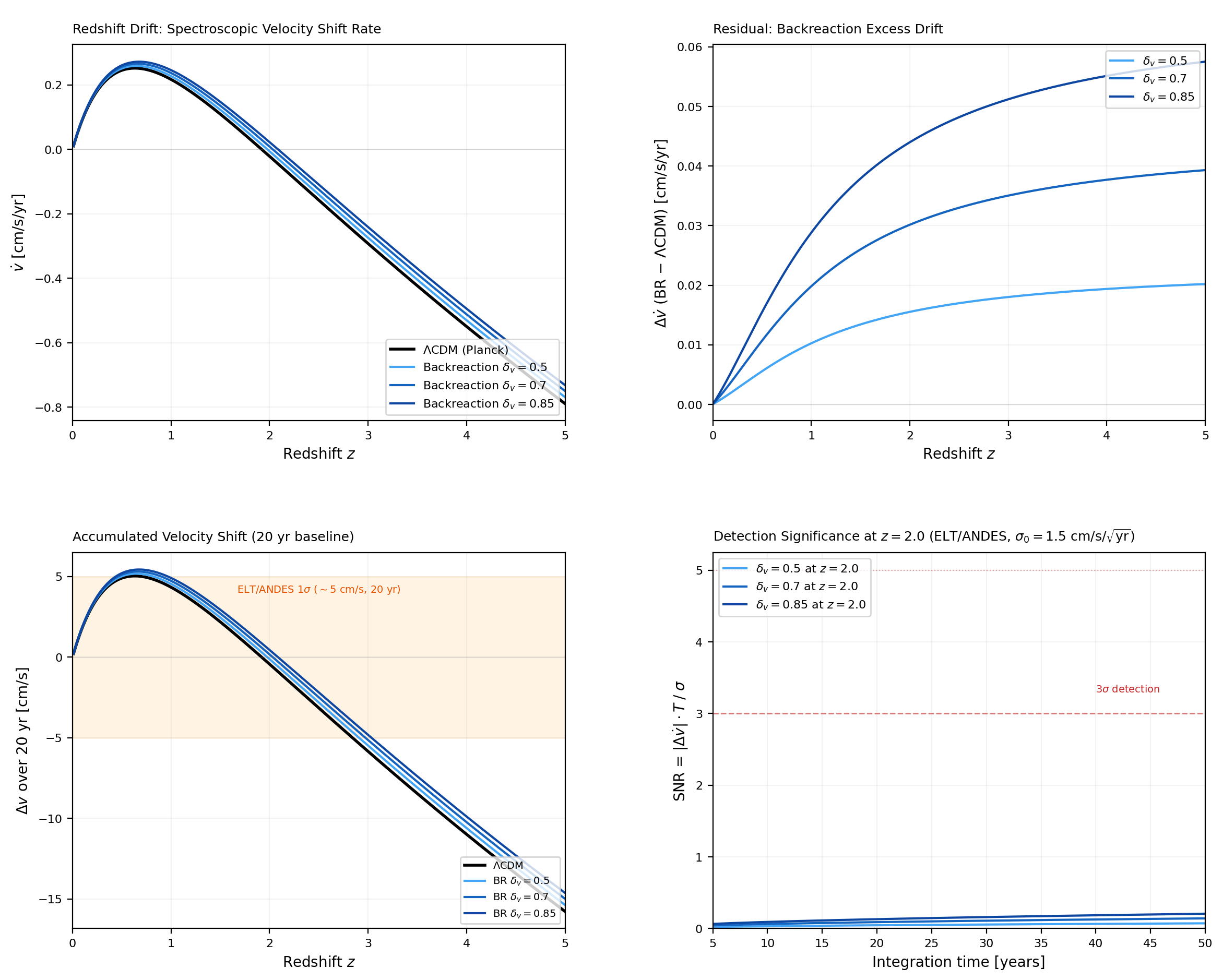
The cosmological redshift drift—the rate at which the redshift of a distant source changes with observer time (Sandage 1962, Loeb 1998)—provides a direct, model-independent measurement of cosmic acceleration:
ż̇ = (1 + z) H0 − H(z)
For the backreaction model, the drift uses a higher local H0 and the structure-corrected HD(z). The expected signal is ~1–5 cm/s over a 20-year baseline, within the projected sensitivity of the ELT/ANDES spectrograph (~1.5 cm/s/√yr for bright QSOs at z ~ 2–4). The backreaction and ΛCDM predictions diverge most at z ~ 2–3, where Lyman-α forest targets are abundant.
Critical Assessment
We address several important limitations of the model:
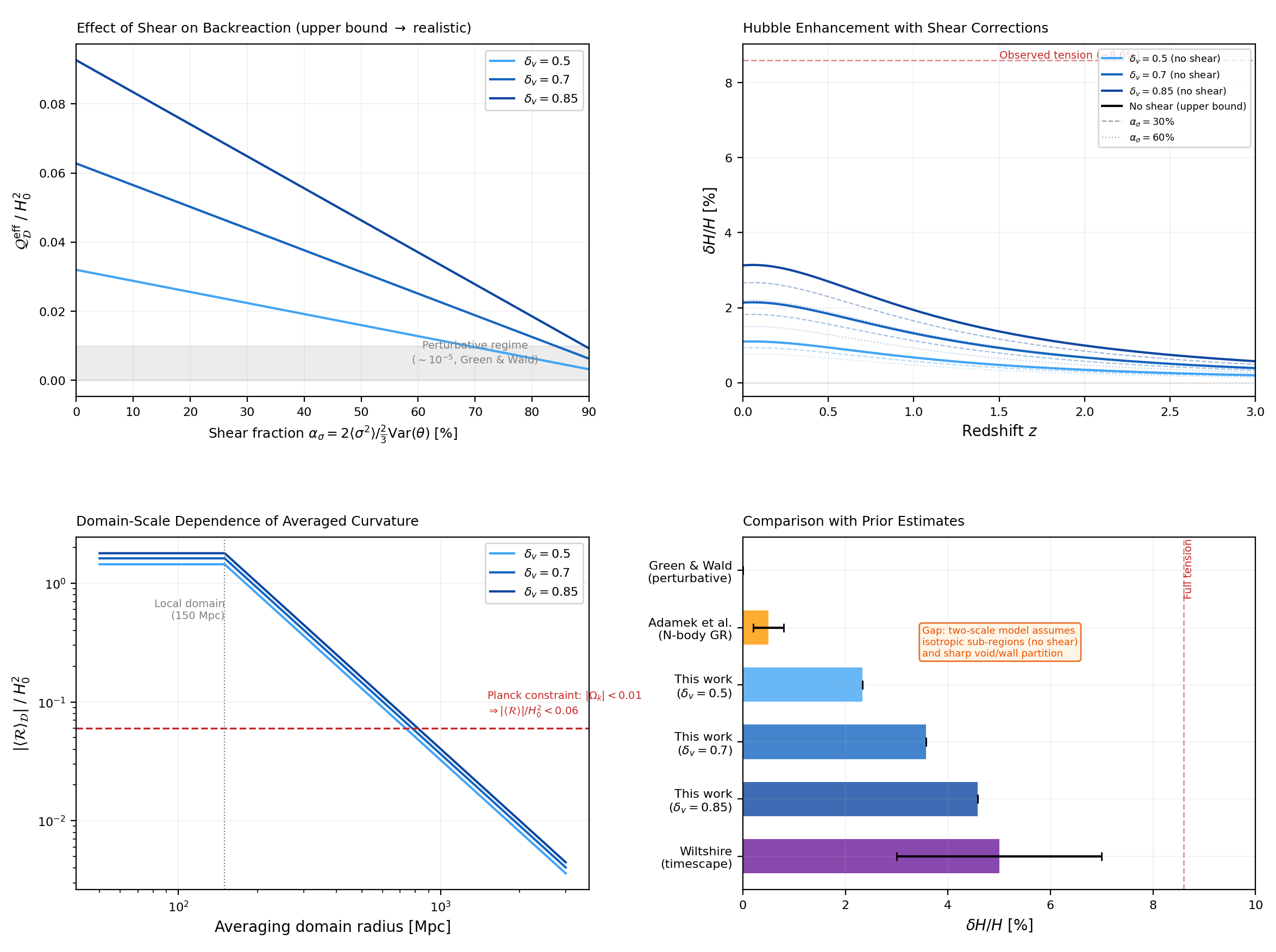
Shear neglect (upper bounds): Real voids are not spherical; filamentary structures produce shear that reduces QD. Our model sets shear to zero for isotropic sub-regions. For realistic cosmic web geometry, the shear fraction ασ ~ 0.3–0.6, reducing QD/H02 from 0.03–0.09 to ~0.01–0.06. Our results should therefore be interpreted as an upper bound.
Domain-local curvature, not global Ωk: Our averaged curvature values ⟨R⟩/H02 ≈ −1.4 to −1.8 correspond to an effective curvature density within the local domain (~150 Mpc). This does not conflict with the Planck CMB constraint |Ωk| ≲ 0.01, which applies to the global curvature averaged over the entire last-scattering surface (~14,000 Mpc). Domain-local curvature dilutes as (Rlocal/Rdomain)2 for larger averaging scales.
Tension with simulations: Our δH/H ≈ 2–5% exceeds the ≲ 0.5–1% found in relativistic N-body simulations (Adamek et al.). With ασ ~ 0.5 shear correction and the observationally viable regime (δv ≲ 0.5), our estimate reduces to δH/H ~ 1–1.5%, in better agreement.
Conclusion
Cosmological backreaction from inhomogeneous expansion is not a speculative proposal—it is a mathematical consequence of averaging the nonlinear Einstein equations. The question is its magnitude.
Main results:
The model yields a kinematical backreaction of QD/H02 ≈ 0.03–0.09, driven primarily by negative averaged spatial curvature from void-dominated geometry. The local Hubble enhancement of δH ≈ 2–5% closes ~25–55% of the Hubble tension. These are upper bounds; with realistic shear corrections, the model provides a ~1–2% correction—reducing the unexplained tension from ~8.6% to ~6–7%.
The model identifies three predictions: (1) a directional H0 anisotropy correlated with the integrated radial tidal field, testable via Pantheon+/2M++ cross-correlation; (2) a redshift drift signature distinguishable from ΛCDM at z ~ 2–3, testable with ELT/ANDES on a 20–30 year baseline; and (3) a structure-enhanced Λ framework that, unlike the Wiltshire timescape, retains the cosmological constant and computes the correction to ΛCDM from inhomogeneous expansion.
The model does not claim to fully resolve the Hubble tension. In the observationally viable regime, it provides a non-negligible correction that standard ΛCDM ignores entirely, but insufficient to resolve the tension on its own. The remaining discrepancy requires additional physics or corrections to measurements related to supernovea in the SH0ES experiment.